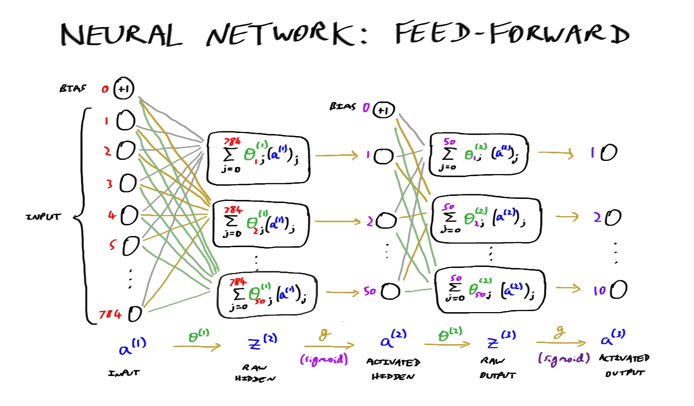
By creating a digit-recognizing neural network - and then writing up the process I followed in order to do so - I was aiming not just to create a working net, but to solidify my understanding of the concepts and calculations involved. Generally speaking, I would say I achieved this.
However, there was one particular step which I found a little mysterious: backpropagation. To quote myself:
The aim of backpropagation is to assess how much of an effect each individual parameter has on the cost function. This is done by calculating the partial derivative of the cost function with respect to each parameter in turn, by feeding back the error from each unit in each layer.
Although I understood the overall principle, at that point I was keen to carry on coding the rest of the network, and I didn’t have the patience or inclination to dive into the underlying maths. In my code I simply used formulae from the internet (cross-checking multiple sources, of course, to establish the correctness of these formulae; during my A-levels, the term we often used for such things was ‘proof by popular consensus’).
I was recently flicking through some notes and doodles I had made over the summer, and came across a page full of partial derivatives, or rather, attempts at them; and I decided it was about time I looked a little deeper into backpropagation.
Note on notation:
- (J()) is the cost function (J) with respect to all parameters () in the net
- (^{(k-1)}) is the set of parameters used to ‘transition’ from layer ((k-1)) to layer (k)
- (z^{(k)}) is the ‘raw’ output from layer (k)
- (a^{(k)}) is the ‘activated’ version of (z^{(k)})
See the diagram at the bottom of the page for a visual representation of how these all relate to each other.

Mission accomplished!
While I had my tablet out, I also thought it might be useful to create a visual representation of the single-hidden-layer network from my earlier project, in order to help me see how the various vectors and matrices fit together:
